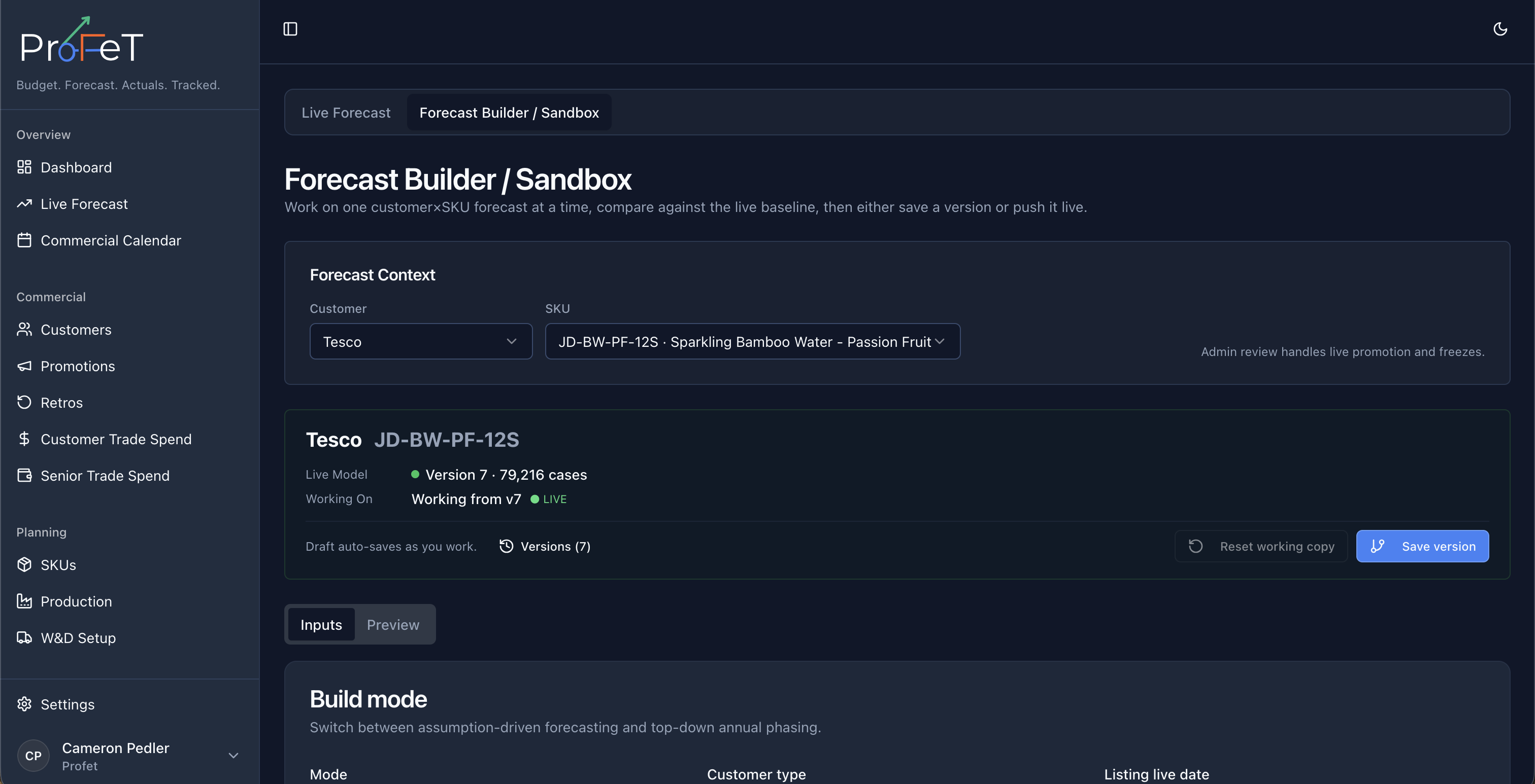
Forecast Builder
Build demand forecasts from market assumptions with real-time volume and P&L projections.
The Forecast Builder lets you model demand for a customer × SKU combination by configuring market assumptions and seeing the resulting volume and financial projections update in real time.
Getting Started
Navigate to Forecast Builder (accessible from the Live Forecast page). Select a Customer and SKU from the dropdowns at the top to begin.
Once both are selected, ProFeT loads any saved assumptions for that pair and immediately calculates a 52-week volume projection.
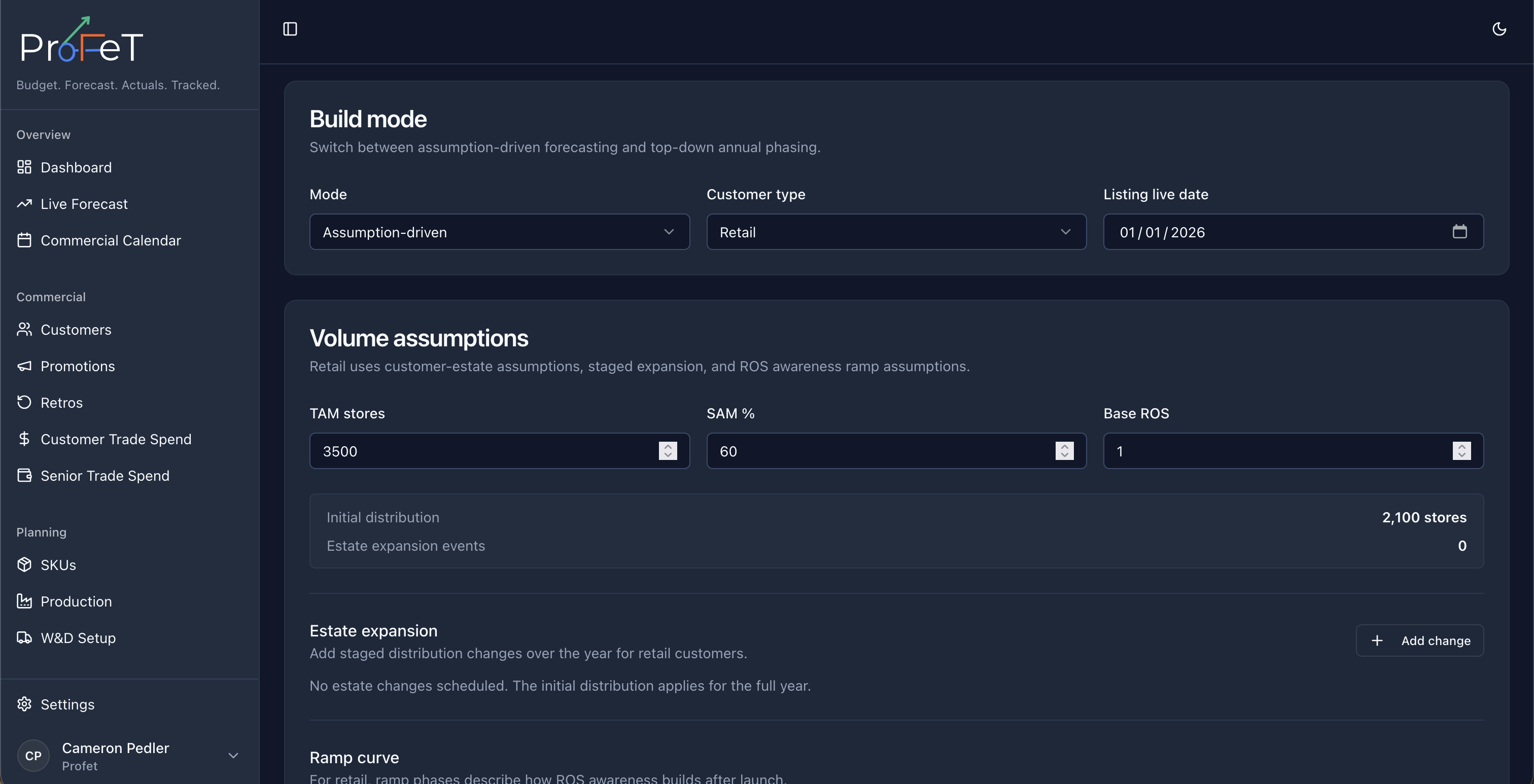
Market Assumptions
These inputs drive the forecast engine. Every change recalculates volumes instantly — no need to click “generate”.
Customer Type
Toggle between Retail and Wholesale. This changes how the ramp curve is interpreted:
- Retail — Ramp represents consumer awareness build. Volume = Active Stores × Base ROS × Ramp% × Seasonality
- Wholesale — Ramp represents account penetration. Volume = (SAM × Ramp%) × Base ROS × Seasonality
Core Inputs
| Input | What it means |
|---|---|
| Total Sites (TAM) | Total addressable market — how many stores or accounts the customer operates |
| SAM % | Serviceable addressable market — what portion is realistically suitable for your product |
| Effective Sites | Derived: TAM × SAM% — the number of sites you’re actually targeting |
| Base ROS | Rate of sale — expected cases per site per week at steady state |
| Listing Live Date | When the product first goes on sale — weeks before this date have zero volume |
Pricing & Costs
| Field | Purpose |
|---|---|
| Price Per Case £ | Selling price — used to calculate GSV |
| COGS Per Case £ | Cost of goods sold — manufacturing cost |
| W&D Per Case £ | Warehousing & distribution cost |
| Retro Per Case £ | Retrospective discount rate |
| Trade Spend Per Case £ | Marketing investment allocated per case |
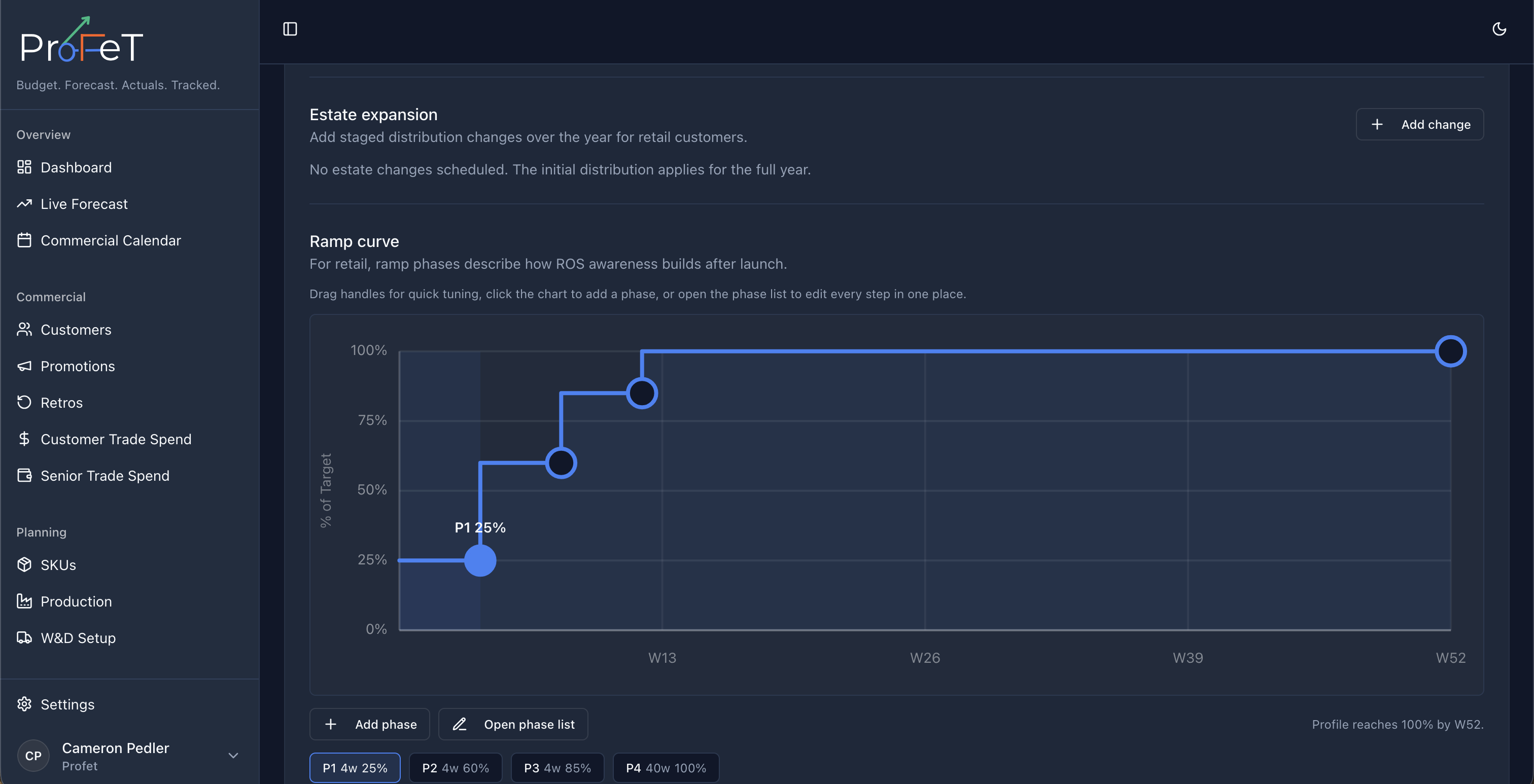
Ramp Curve
The ramp curve models how quickly sales build after listing. It’s defined as a series of phases, each with a duration (weeks) and a percentage (0–100%).
Example:
- Phase 1: 4 weeks at 25% — initial launch period
- Phase 2: 8 weeks at 50% — growing awareness
- Phase 3: 12 weeks at 75% — approaching steady state
- Phase 4: 28 weeks at 100% — full run rate
Click the visual editor to drag points on an interactive chart, or edit the table directly. Add/remove phases as needed.
For wholesale customers, there’s also a Peak Penetration % slider that caps the maximum percentage of SAM that will ever be reached.
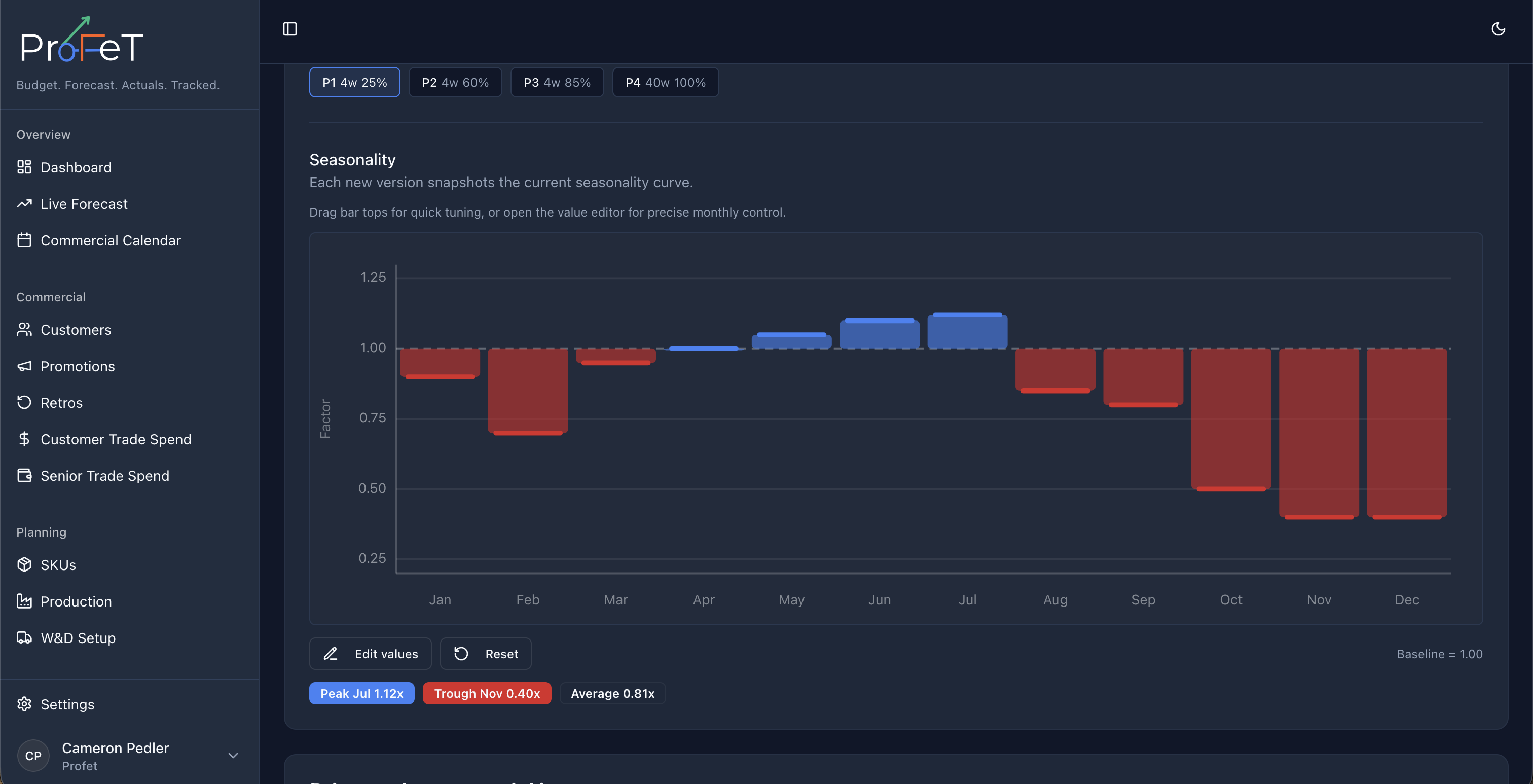
Seasonality
Twelve monthly multipliers (Jan–Dec) that adjust volume for seasonal demand patterns. A value of 1.0 means no adjustment. Values above 1.0 increase demand; below 1.0 decrease it.
- Reset to Flat sets all months to 1.0
- Load Category Defaults pulls seasonality from the SKU’s product category (if configured)
Estate Expansion (Retail only)
For retail customers, you can schedule store count changes over the year — e.g. “from week 13, increase to 250 stores” to model new store openings or closures. Each change affects the volume projection from that week onwards.
Promotional Uplift
ProFeT automatically matches active promotions for the selected customer and SKU. Any promotion with a date range overlapping the forecast period applies a volume uplift.
If multiple promotions overlap in the same week, the highest uplift wins (not additive — this prevents over-inflating demand).
Volume Output
Weekly Cases
A 52-row table showing the calculated cases per week. You can click any cell to override the calculated value with a manual number. Overridden cells are highlighted in amber.
Overrides are useful for one-off adjustments — e.g. a known order, a distribution pause, or a promotional event that the model doesn’t capture.
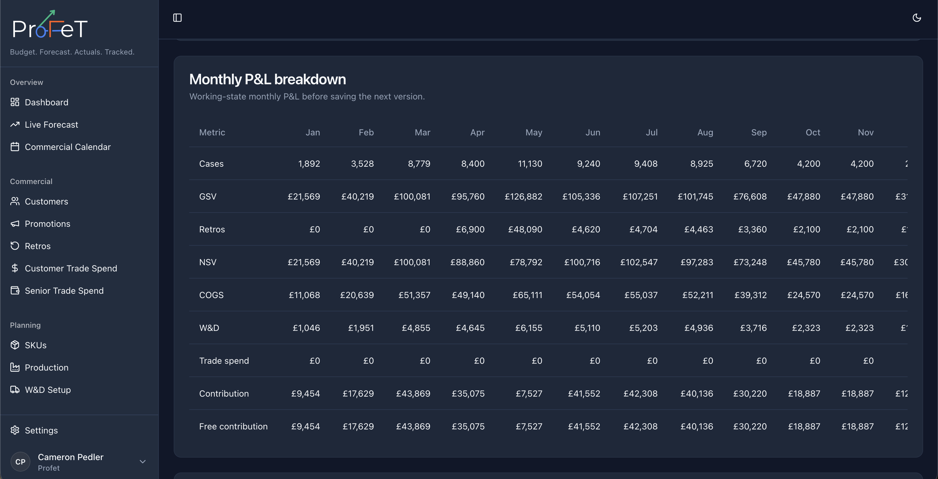
Monthly Summary
Aggregates weekly volumes into 12 months, showing total cases per month alongside a bar chart.
Annual Total
The big number at the top — your total forecast cases for the year.
P&L Preview
The financial cascade computed from your volumes and pricing inputs:
Cases × Price/Case           = GSV (Gross Sales Value)
GSV − Retros                 = NSV (Net Sales Value)
NSV − COGS − W&D             = Contribution
Contribution − Trade Spend   = Free Contribution
Shown as:
- Waterfall strip — colour-coded cards showing each step
- Monthly P&L table — month-by-month breakdown of all metrics
Comparison P&L
Compare your working forecast against a baseline — either the current live forecast or a saved snapshot. Shows deltas and percentage changes for each metric, colour-coded (green = favourable, red = unfavourable).
Sensitivity Analysis
See the impact of ±10% and ±20% changes to ROS and Price on your volumes and margins. Useful for stress-testing assumptions.
Scenarios
Scenarios let you maintain multiple assumption sets for the same customer × SKU without overwriting your work.
Example use cases:
- “Base Case” vs “Optimistic” vs “Conservative”
- “With new listing” vs “Without”
- “Current pricing” vs “Price increase”
Each scenario stores its own complete set of assumptions (sites, SAM, ROS, ramp, seasonality, pricing).
Creating a Scenario
Click New Scenario in the Scenarios & Versions panel. Give it a name — your current assumptions are saved automatically.
Switching Scenarios
Click Select on any scenario to load its assumptions into the editor. The volume and P&L projections update immediately.
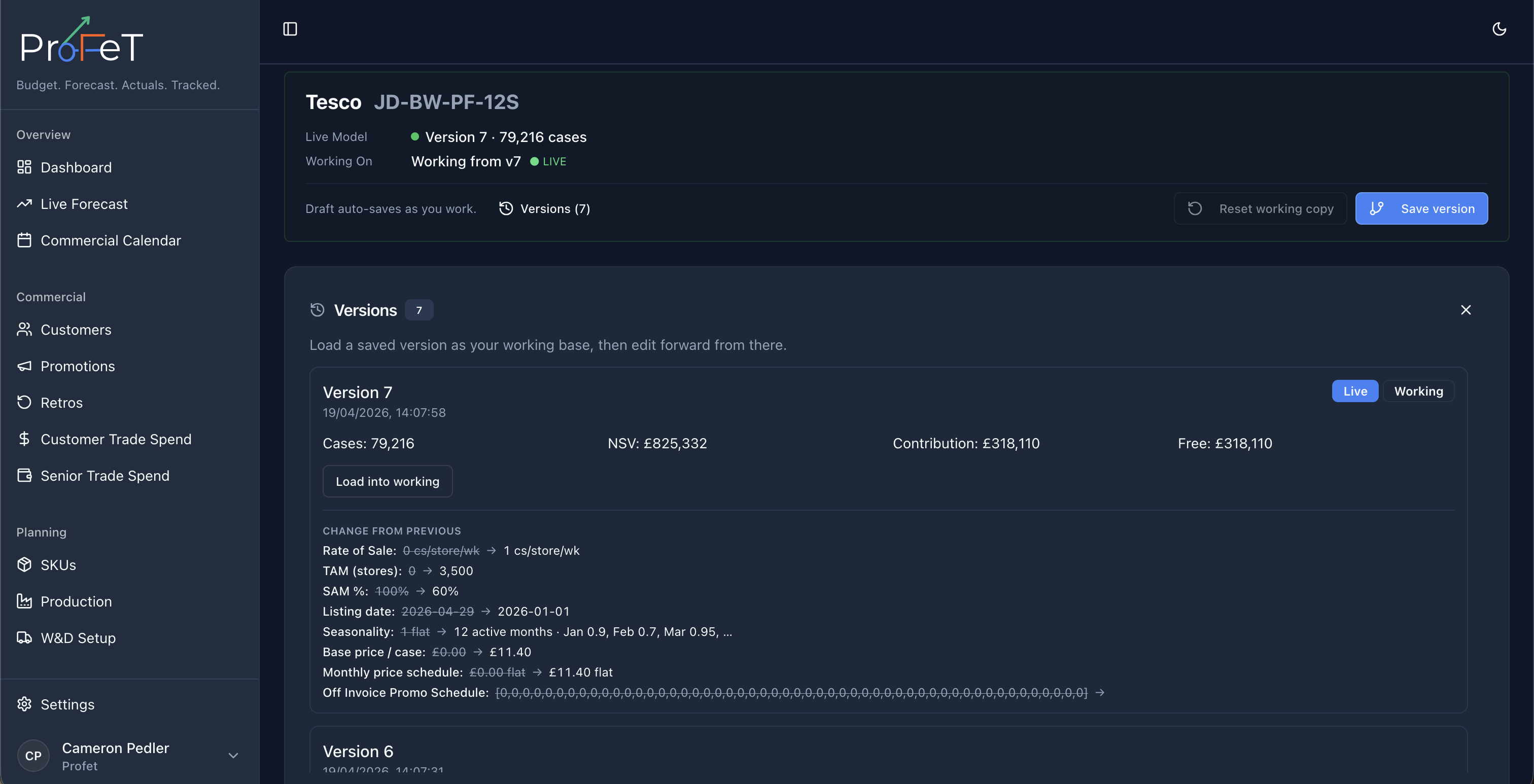
Versions
Versions are point-in-time snapshots saved within a scenario. They capture:
- All volume assumptions
- Computed weekly and monthly volumes
- P&L totals (cases, NSV, contribution)
Saving a Version
Click Save Version in the header. Give it a name and optional notes describing what changed.
Locking a Version
One version can be locked as the official live plan. Click Make Live on any version in the history. This:
- Unlocks any previously locked version
- Sets the selected version as the authoritative forecast
- Makes it available as the comparison baseline
Change Log
Tracks every assumption change you make during the current session — field name, old value, new value, and timestamp. Useful for reviewing what you changed before saving.
Debug Panel
For advanced users. Shows the per-week calculation breakdown from the ROS engine: sites, ramp%, base ROS, seasonality multiplier, promo uplift, base volume, and final volume. Helpful for understanding exactly why a particular week has the volume it does.
Saving Your Work
- Save Assumptions — Persists the current assumptions to the API for this customer × SKU pair
- Save Version — Creates a named snapshot you can return to later
- Generate & Submit — Validates the forecast and submits it for review on the Live Forecast page
Forecast Builder Screens